
Building Production-Grade RAG Systems with Elasticsearch
A technical blueprint for engineers building RAG at production scale with hybrid search, vector quantization, and agentic AI

This blog post was submitted to the Elastic Blogathon Contest and is eligible to win a prize.
01 — The Hallucination Hurdle: Why Search Alone Falls Short
LLMs are impressive at one specific thing: synthesizing fluent text from patterns they memorized during training. That capability becomes dangerous the moment someone deploys them against real business questions. They have no access to your private data, no awareness of what changed last Tuesday, and no mechanism for saying “I don’t know.” Instead they guess — and they do it with the confidence of someone who absolutely should know. That’s the hallucination problem in plain terms.
Keyword search is the other half of the same problem. BM25 is a beautifully precise algorithm for what it does — matching tokens — but tokens are a brittle proxy for intent. Search for “heart attack” and miss every document about “myocardial infarction.” Search for “cost reduction” and skip the entire “expense optimization” folder. Lexical retrieval has no model of meaning; it only knows about character sequences.
Retrieval-Augmented Generation (RAG) solves this by providing the LLM with grounded context before it generates anything. Elasticsearch retrieves the most relevant, up-to-date passages from your private data. Those passages become the model’s evidence. The LLM’s job shifts from “recall and invent” to “synthesize from what’s in front of you.”
💡 Prompt engineering cannot fix a retrieval problem. If your model doesn’t have accurate evidence in its context window, no instruction will conjure it. RAG is an infrastructure decision, not a model configuration.
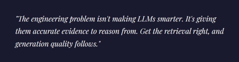
02 — Why Elasticsearch for RAG?
Choosing a vector database feels like an infrastructure decision but it’s actually a product decision. Pinecone gets you to a demo in an afternoon. Then you need to filter by department and date. Then you need field-level security for compliance. Then your ops team asks why there’s no trace when retrieval quality drops. Purpose-built vector stores tend to be excellent at the narrow thing they were designed for, and increasingly painful for everything else.
Elasticsearch’s decisive advantage is that it was never just a search engine. It’s a distributed analytics platform that happens to have world-class vector capabilities. You get hybrid search, geospatial filtering, time-series aggregation, field-level security, and a decade of operational battle-testing — all in one platform.
03 — Hybrid Search & Reciprocal Rank Fusion
The most important architectural decision in any RAG system is your retrieval strategy. Semantic search alone misses exact technical terms. Keyword search alone misses conceptual intent. The production-proven solution is Reciprocal Rank Fusion (RRF) — a mathematically elegant algorithm for merging ranked lists from disparate retrievers without needing score normalization.
The formula: for each document, sum 1/(k + rank) across all retrievers, where k=60 is a smoothing constant that prevents any single top-ranked result from dominating. Documents that rank well in both BM25 and vector search win.
POST /enterprise-knowledge/_search
{
  "sub_searches": [
    {
      "query": { "match": { "content": "distributed consensus algorithm" } }
    },
    {
      "knn": {
        "field": "content_vector",
        "query_vector_builder": {
          "text_embedding": {
            "model_id": "openai-embeddings",
            "model_text": "distributed consensus algorithm"
          }
        },
        "k": 10,
        "num_candidates": 100
      }
    }
  ],
  "rank": { "rrf": { "window_size": 100, "rank_constant": 60 } }
}
💡 Why not score normalization? BM25 scores and cosine similarity live in completely different numerical ranges. RRF sidesteps this entirely by operating on ranks, not scores. It’s robust, parameter-light, and empirically superior to linear combination methods.
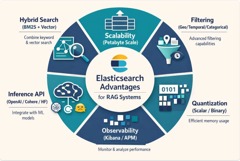
04 — Vector Quantization: From float32 to Single Bits
At production scale, RAM is your most constrained resource. A 1-million-vector index at float32 (1536 dimensions) consumes roughly 6GB of RAM — just for the vectors, before indexing overhead. Multiply to 1 billion vectors and infrastructure costs become untenable.
Elasticsearch’s quantization hierarchy gives engineers a precise dial between memory cost and retrieval fidelity:
bfloat16 → 2× memory reduction 2 bytes/value instead of 4. Maintains float32’s dynamic range with reduced mantissa precision. Near-zero recall penalty.
Scalar int8 → 4× memory reduction 32-bit floats compressed to 8-bit integers. Minimal accuracy loss in most enterprise RAG workloads.
int4 Scalar → 8× memory reduction 4-bit integer quantization. Requires rescoring with original vectors for precision-critical applications.
BBQ (Better Binary Quantization) → 32× memory reduction Single-bit compression. SIMD Hamming distance replaces float math. Breakthrough for 2025/2026 deployments at massive scale.
PUT /enterprise-knowledge
{
  "mappings": {
    "properties": {
      "content": { "type": "text" },
      "content_vector": {
        "type": "dense_vector",
        "dims": 1536,
        "index": true,
        "similarity": "cosine",
        "index_options": {
          "type": "bbq_hnsw",
          "confidence_interval": 0.99
        }
      }
    }
  }
}
05 — DiskBBQ: Eliminating the Latency Cliff
Even with BBQ reducing memory 32×, billion-scale workloads can still exceed your RAM budget. Traditional HNSW indexes suffer from a brutal failure mode: once available RAM is exhausted, the OS begins swapping index segments to disk and latency jumps from milliseconds to seconds.
DiskBBQ redesigns retrieval around disk-friendly access patterns using Hierarchical K-means clustering:
Centroid Query — The query vector is compared against compact cluster centroids in memory, identifying the 2–3 most relevant partitions on disk.
Selective Cluster Loading — Only those partitions are loaded from disk. Sequential disk reads are fast; random reads (HNSW’s pattern) are slow.
Bulk In-Memory Scoring — Candidates are scored using SIMD-accelerated Hamming distance. Top-K returned with optional float32 rescoring.
FormatRAM (1M Vectors)LatencyBuild TimeHNSW float32~4–6 GB< 5msStandardHNSW BBQ~150–200 MB~3.4msFastDiskBBQ~100 MB~4–15ms10× Faster
06 — Chunking: The Most Underrated Engineering Decision
No retrieval algorithm compensates for poor chunking. Chunks too small lose surrounding context. Chunks too large introduce noise that dilutes the LLM’s answer and burns tokens.
Recursive Paragraph Splitting — Uses a hierarchy of separators (\n\n → \n → space) to split on natural document boundaries. Paragraphs and sentences stay together wherever possible.
Semantic Chunking — Computes embedding similarity between consecutive sentences. A chunk boundary is inserted only when a significant topical shift is detected. Empirically improves retrieval precision by 15–25% over fixed-size approaches.
Hierarchical Parent-Child Indexing — The architecture pattern that resolves the tension between retrieval and generation:
Child chunks (200–400 tokens) — optimized for precise vector matching
Parent chunks (800–1000 tokens) — optimized for comprehensive LLM context
At query time: search the child index for precision, then use parent_id pointers to fetch the full parent chunk as LLM context. Surgical retrieval, rich generation.
def ingest_hierarchical(document_text, metadata):
    parent_chunks = split_recursive(document_text, chunk_size=900)

    for parent in parent_chunks:
        parent_id = str(uuid.uuid4())

        # Store parent (not vectorized)
        es.index(index="parent-chunks", id=parent_id,
                 document={"content": parent, "metadata": metadata})

        # Split into child chunks and vectorize
        for child in split_recursive(parent, chunk_size=300):
            es.index(index="child-chunks", document={
                "content": child,
                "parent_id": parent_id,
                "content_vector": model.encode(child)
            })
07 — ColPali & Late Interaction: Searching What You Can See
A large fraction of enterprise knowledge lives in visually rich formats: PDFs with charts, scanned forms, engineering diagrams. Traditional RAG routes these through OCR — which fails silently on complex layouts and completely drops visual-only information.
ColPali and ColBERT take a different approach. Instead of compressing a document into a single vector, late interaction models generate a separate vector for every token or visual patch. Full semantic granularity is preserved until the final matching stage using the MaxSim operator — for each query token, find its maximum similarity against any document token, then sum across all query tokens.
Production implementation in two stages:
First stage — Average vector ANN search over 1 vector per document to retrieve top 50–100 candidates cheaply
Second stage — Full MaxSim reranking over all patch vectors of candidates for high-precision results
Elasticsearch 8.18+ supports multi-vector representations via the rank_vectors field type.
💡 Using models like CLIP or ImageBind, Elasticsearch can map text, images, audio, and video into a unified latent space. A text query directly retrieves relevant images or audio clips — no transcription pipeline required.
08 — Agentic AI & the Model Context Protocol
The next evolution of RAG systems isn’t a better retrieval algorithm — it’s giving AI agents the autonomy to figure out what to retrieve. The Elastic Agent Builder formalizes this with a four-phase reasoning loop:
A. Index Discovery — Using the index_explorer tool, the agent identifies which of potentially thousands of indices are relevant. This eliminates an entire category of retrieval errors.
B. Schema Understanding — The agent inspects index mappings to understand field names and types. It constructs type-safe queries rather than guessing schema structure.
C. Query Generation & Execution — The agent writes valid Query DSL or ES|QL, executes it, and evaluates whether results are sufficient.
D. Iterative Synthesis — If the answer is incomplete, the agent reformulates — different fields, filters, or query types — until it reaches a high-confidence response.
Model Context Protocol (MCP) is the open standard that exposes Elasticsearch as standardized tools any LLM can call — list_indices, get_mappings, search, esql — enabling Claude, GPT-4o, or any MCP-compatible model to query your data directly without custom API wrappers.
09 — GPU Acceleration & Observability
HNSW graph construction is the most compute-intensive phase of the vector pipeline. Elasticsearch 9.x integrates NVIDIA cuVS to offload this to the GPU:
12× indexing throughput — Re-index billion-scale datasets in hours, not days
7× force-merge speed — Faster index optimization windows
CPU freed for search — Graph construction moves to GPU, freeing CPU cycles for query handling under concurrent load
For observability, standard application monitoring cannot capture RAG-specific failures: retrieval precision degradation, embedding drift, context window overflow, or faithfulness regressions. Use dedicated tools:
Ragas — Automated metrics: context precision, recall, faithfulness, answer relevance
Arize Phoenix — Embedding drift detection and retrieval quality monitoring
LangSmith — Deep trace visibility for LangChain pipelines
Langfuse — Self-hostable, open-source, multi-turn conversation support
10 — Case Studies: Uber & DoorDash
Uber — Project Sunrise Uber migrated their proprietary “Sia” search platform and ingested 1.5 billion items in 2.5 hours — 79% faster than baseline. Their key innovation: Matryoshka Representation Learning (MRL), producing embeddings that can be truncated at different dimensions, letting different applications trade retrieval quality for latency without separate models. P99 latency target: 100ms at 2K QPS.
DoorDash — LLM Guardrails DoorDash’s Dasher support chatbot uses RAG with a real-time guardrail that evaluates responses before they reach users. An LLM Judge scores every response across five axes: retrieval correctness, response accuracy, grammar, coherence to context, and relevance. Non-compliant responses are intercepted and regenerated or escalated to human support.
Production Engineering Checklist
Implement hybrid search with RRF combining BM25 and kNN
Use bfloat16 or int8 HNSW quantization as your starting point
Deploy DiskBBQ when your vector corpus exceeds available RAM
Use semantic or recursive paragraph chunking with 10–15% token overlap
Decouple retrieval chunk size (200–400 tokens) from generation chunk size (800–1000 tokens)
Use ColPali for PDFs, charts, and scanned documents — skip OCR
Expose Elasticsearch via MCP for autonomous agent access
Deploy NVIDIA cuVS for bulk ingestion and reindexing pipelines
Integrate Ragas to measure context precision, recall, and faithfulness
Instrument every step of the pipeline — you cannot debug what you cannot trace
Conclusion
Ten years ago a database was infrastructure. Something you provisioned, backed up, and largely ignored. Today, retrieval quality directly determines whether your AI product is useful or embarrassing. The stack described in this guide — from BBQ quantization to DiskBBQ to ColPali to MCP-powered agents — exists because the industry collectively hit the limits of naive vector search and had to engineer its way out.
Elasticsearch earned its position in this stack the hard way — through a decade of production deployments across every scale and domain. The vector capabilities are new. The operational maturity is not. That combination is genuinely hard to replicate.
Retrieval is not a supporting act. It is the show.